Z 4 Z 3 Z 2 Z 1 0
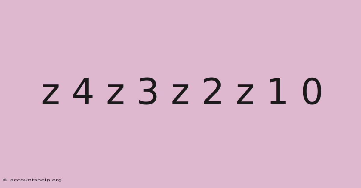
The Pattern That Broke My Brain
I still remember the first time I saw it written down. Even so, or maybe a recipe. Practically speaking, not as a formula, not as a theorem — just scrawled on a napkin during a late-night coffee shop conversation between two engineers who were clearly arguing about something I didn't understand. But something about those symbols — z₄ z₃ z₂ z₁ 0* — stuck with me. It looked like a code. Or maybe the beginning of a very specific kind of mathematical poetry.
Turns out, it wasn't either of those things. But it was something far more interesting: a window into how engineers and mathematicians think about systems, signals, and structure. If you've ever wondered what all those subscripts mean, or why someone would write a sequence that ends in zero, stick around. This is one of those ideas that seems impossibly abstract until it clicks — and then suddenly you start seeing it everywhere.
What Is z₄ z₃ z₂ z₁ 0?
Let's be honest: if you Google "z₄ z₃ z₂ z₁ 0," you won't find a Wikipedia page. There's no single, canonical definition. So what you will* find — if you dig into digital signal processing textbooks, control theory papers, or certain corners of electrical engineering forums — is a notation pattern. Now, a shorthand. A way of writing a polynomial or a sequence where each term is labeled by its position or index, and the last term is zero.
In the context of digital filters, for example, z₄ z₃ z₂ z₁ 0* might represent the taps of a finite impulse response (FIR) filter, where each zₙ is a coefficient applied to a delayed version of the input signal. The "0" at the end? That's the current sample — no delay. It's the anchor point.
In polynomial algebra, it could be the descending powers of a variable: z⁴ + z³ + z² + z¹ + z⁰*, where z⁰ = 1*. The zero isn't nothing — it's the constant term. The foundation.
In control systems, this notation often appears in the context of the Z-transform, a tool used to analyze discrete-time signals. The z⁻ⁿ terms represent delays, and the arrangement of coefficients tells you how the system responds to inputs over time.
The short version? z₄ z₃ z₂ z₁ 0* isn't a thing you can look up. That said, it's a pattern you recognize. And once you do, it shows up in surprising places.
The Z-Transform Connection
If you've studied signals and systems, you've probably seen the Z-transform written as:
X(z) = Σ x[n] z⁻ⁿ
That z⁻ⁿ term is doing a lot of work. In practice, it represents a delay. z⁻¹ means "one sample ago." z⁻⁴ means "four samples ago." So when someone writes z₄ z₃ z₂ z₁ 0*, they might be shorthand-ing a transfer function where the coefficients are arranged by delay order, and the "0" represents the present moment — the undelayed term.
This is the kind of notation that lives in whiteboard sketches and lecture slides, not in formal papers. It's how people think* about systems, not how they publish them.
Why the Zero Matters
The trailing 0 is the most interesting part. Which means in a filter, it's the coefficient for the current input sample. In a polynomial, z⁰ = 1*, so it's the constant term. Practically speaking, in a delay line, it's the "now" tap. It's the reference point from which everything else is measured.
Without it, you're working in a world of pure delay — echoes with no source. With it, you have a system that can respond to the present moment.
Why It Matters / Why People Care
Here's the thing about z₄ z₃ z₂ z₁ 0* — it's not just notation. It's a mindset. It represents the way engineers and mathematicians break down complex systems into ordered, indexed components. And that way of thinking? It's everywhere.
In Digital Audio
Every time you adjust an EQ setting on your phone, you're interacting with a system built on this kind of indexing. The bass boost? That's a low-pass filter with coefficients arranged like z₄ z₃ z₂ z₁ 0*. The treble cut? In real terms, a high-pass filter. Consider this: the reverb? A network of delays, each one a z⁻ⁿ term.
The reason your headphones can simulate a concert hall in a 200-millisecond impulse response is because someone figured out how to arrange coefficients in just the right pattern — a pattern that looks a lot like z₄ z₃ z₂ z₁ 0*.
In Control Systems
When a drone stabilizes itself in flight, when a thermostat maintains your room temperature, when a car's cruise control adjusts to maintain speed — all of these systems rely on feedback loops where past errors are weighted and combined with current measurements. That weighting? It's z₄ z₃ z₂ z₁ 0*.
The "0" is the proportional term — how hard you push based on the current error. The z₁, z₂, z₃, z₄* terms are the integral and derivative actions — how you account for accumulated past behavior and predicted future trends.
In Machine Learning
Believe it or not, this pattern shows up in recurrent neural networks (RNNs) and their more sophisticated cousins. Here's the thing — when an RNN processes a sequence, it maintains a hidden state that's updated based on the current input and the previous state. The update rule often involves weighted combinations of past states — indexed, ordered, and anchored by the present.
This is one of those details that makes a real difference.
z₄ z₃ z₂ z₁ 0* is, in a sense, the DNA of sequential processing. It's how you build memory into a system.
How It Works (or How to Do It)
Let's get concrete. If you want to understand z₄ z₃ z₂ z₁ 0*, the best way is to build something with it. Here's how I'd walk a beginner through it.
Step 1: Understand the Indexing
The subscripts aren't arbitrary. z₁ is the most recent past. z₄ is the oldest term. They tell you the order. 0 is the present.
... z₄  z₃  z₂  z₁  [0]
    -4  -3  -2  -1   now
Each zₙ represents a sample taken n time steps in the past. The "0" is the current sample.
If you found this helpful, you might also enjoy equation for newton's universal law of gravitation or is 91 a composite or prime number.
Step 2: Assign Coefficients
In practice, each position gets a weight. A simple moving average filter might look like this:
y[n] = (1/5) * (x[n] + x[n-1] + x[n-2] + x[n-3] + x[n-4])
In z notation, this is:
Y(z) = (1/5) * (1 + z⁻¹ + z⁻² + z⁻³ + z⁻⁴) * X(z)
The coefficients are all 1/5, and the z terms go from z⁰ (which is 1) to z⁻⁴. If you write them in descending order of delay, you get something that looks like z₄ z₃ z₂ z₁ 0* — except here the subscripts are negative exponents.
Step 3: Implement It
In code, this becomes a simple loop:
def moving_average(x, window=5):
    y = []
    for n in range(len(x)):
        total = 0
        count = 0
        for k in range(min(window, n + 1)):
            total += x[n - k]
            count += 1
        y.append(total / count)
    return y
The k index here is essentially your z₄ z₃ z₂ z₁ 0* pattern. Each iteration looks back at the previous samples, weighted by their position.
Step 4: Analyze Stability
Here's where it gets
Step 4: Analyze Stability
When you start looking at the z‑domain representation, stability becomes a question of where the poles of the transfer function lie. For the moving‑average filter above the transfer function is
[ H(z)=\frac{1}{5}\bigl(1+z^{-1}+z^{-2}+z^{-3}+z^{-4}\bigr) ]
Because every pole is at the origin (the denominator is just 1), the filter is inherently stable — no matter how long the window, the response cannot blow up.
Contrast that with a recursive filter such as a simple IIR low‑pass:
[ H(z)=\frac{1}{1-a z^{-1}},\qquad |a|<1 ]
Here the pole sits at (z = a). If (|a|\ge 1) the pole would move outside the unit circle and the output would diverge for any non‑zero input. The z₄ z₃ z₂ z₁ 0* pattern reminds us that each past sample is multiplied by a coefficient that corresponds to a specific delay; the collection of those delays forms a polynomial whose roots dictate whether the system will settle or run away.
In practice, engineers plot the poles on the complex plane (the z‑plane) and verify that they all reside strictly inside the unit circle. That visual check is the bridge between the abstract z notation and concrete design constraints.
Step 5: From Theory to Real‑World Applications
1. Digital Controllers
In a PID controller implemented on a microcontroller, the discrete‑time version of the derivative term is often expressed as
[ K_d \frac{e[n]-e[n-1]}{T_s} ]
If you expand the error sequence into a longer history, you end up with a weighted sum that looks exactly like z₄ z₃ z₂ z₁ 0* — the derivative coefficient multiplies the most recent difference, the integral coefficient accumulates older differences, and the proportional term sits at the present sample.
2. Audio Effects
Reverberation algorithms model sound reflections as a series of decaying echoes. Each echo is a delayed, attenuated replica of the original signal, which can be written as
[ y[n]=\sum_{k=0}^{N} \alpha_k , x[n-k] ]
When the coefficients (\alpha_k) are chosen to mimic the exponential decay of a physical space, the resulting filter’s transfer function is a rational function whose numerator encodes the z₄ z₃ z₂ z₁ 0* pattern of delays.
3. Time‑Series Forecasting
ARIMA models (AutoRegressive Integrated Moving Average) are essentially linear combinations of past observations and past prediction errors. The AR part is a direct embodiment of z₄ z₃ z₂ z₁ 0*: each lagged term is multiplied by a weight that corresponds to its position in the history.
Step 6: Practical Tips for Working With z₄ z₃ z₂ z₁ 0*
| Tip | Why It Matters |
|---|---|
| Normalize coefficients so that the sum equals 1 for filters that should preserve DC gain. Think about it: | |
| Use floating‑point arithmetic for the first few iterations when testing a new filter. | Makes it feasible to work with deep z‑delay lines on embedded hardware. |
| Validate with a step response before deploying. In real terms, | Prevents unintended scaling of the output. In real terms, |
| Check the pole‑zero map after designing a filter. | Avoids hidden overflow or underflow that can corrupt the early samples. |
| Implement a circular buffer for long histories to keep memory usage bounded. | Lets you see whether the system settles as expected or exhibits overshoot/oscillation. |
Conclusion
The notation z₄ z₃ z₂ z₁ 0* may look like a cryptic string of symbols, but at its core it encodes a universal principle: any system that evolves over time can be described as a weighted sum of past states, anchored to the present. Whether you are tuning a cruise‑control loop, designing a digital filter, or building a recurrent neural network, you are implicitly manipulating the same set of delayed terms — just with different names and different domains.
Understanding the z‑domain gives you a powerful lens through which to view stability, frequency response, and design trade‑offs. And by translating the abstract z₄ z₃ z₂ z₁ 0* pattern into concrete coefficients, visual pole maps, and testable code, you turn a theoretical construct into a practical tool. The bottom line: mastering this pattern equips you to predict how a system will behave, to shape that behavior deliberately, and to troubleshoot it when things go awry — making it a cornerstone of modern engineering across control, signal processing, and machine learning.
Latest Posts
Recently Shared
-
What Is The Basic Function Of Hydrostatic Pressure
Aug 01, 2026
-
What Is The Lewis Structure Of Brf5
Aug 01, 2026
-
Chemical Reaction Between Hcl And Naoh
Aug 01, 2026
-
Points On The Same Line Are Called
Aug 01, 2026
-
What Is The Definition Of Gravitational Energy
Aug 01, 2026
Related Posts
We Picked These for You
-
Which Is A Non Membrane Bound Organelle
Aug 01, 2026
-
How To Solve For Limiting Reagent
Aug 01, 2026
-
How Many Electrons In The F Orbital
Aug 01, 2026
-
Length Of Segment Of Circle Formula
Aug 01, 2026
-
What Type Of Tissue Is Avascular
Aug 01, 2026
