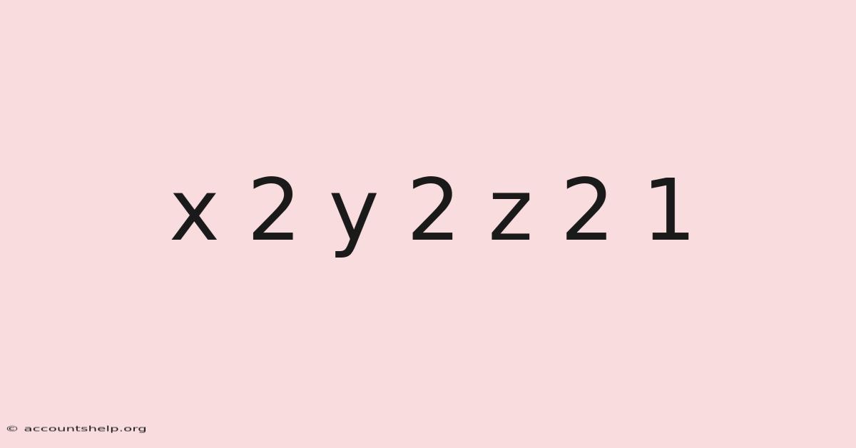
You're staring at a formula you've seen a hundred times. x² + y² + z² = 1. In real terms, clean. Symmetric. Almost boring on a whiteboard That's the part that actually makes a difference. Turns out it matters..
But here's the thing — this single equation describes every point on the surface of a perfect sphere with radius 1, centered at the origin. Every quantum state on the Bloch sphere. Every directional vector in 3D graphics. That's why every satellite orbit. They all live on this surface Surprisingly effective..
And most people who "know" this equation have never actually worked with it.
What Is x² + y² + z² = 1
At its core, this is the distance formula in three dimensions, set equal to a constant Small thing, real impact..
In two dimensions, x² + y² = 1 gives you a unit circle. Now, add the z term and you've extruded that circle into a sphere. So every point (x, y, z) that satisfies the equation sits exactly one unit from the origin. No more, no less.
The geometric meaning
Picture a sphere floating in space, centered at (0, 0, 0). Its radius is 1. Its diameter is 2. Also, its surface area is 4π. Its volume is 4π/3.
The equation doesn't describe the interior — that would be x² + y² + z² ≤ 1. That said, it describes only the skin. The boundary. A 2D surface embedded in 3D space.
This distinction matters more than most textbooks let on It's one of those things that adds up..
Why "unit" matters
Radius 1 isn't arbitrary. It's the normalization standard. Any sphere of radius r can be scaled to this one by dividing coordinates by r. Any vector can be normalized to length 1 by dividing by its magnitude.
When you see a direction vector in a graphics shader or a physics simulation, it almost always lives on this sphere. Not inside it. On it The details matter here..
Why It Matters / Why People Care
You might encounter this equation in a calculus III final and forget it by Tuesday. But it keeps showing up in places that actually ship code, launch hardware, or model reality.
Computer graphics and game engines
Every normal map. Every environment map lookup. Every reflection vector calculation. They all assume unit vectors — points on this sphere.
When a fragment shader computes lighting, it dots the surface normal against the light direction. Both are unit vectors. So both live on x² + y² + z² = 1. If either drifts off the sphere due to floating-point accumulation or bad interpolation, lighting breaks. Day to day, specular highlights flicker. Reflections warp.
This is why normalize() exists. It projects any non-zero vector back onto the unit sphere.
Quantum computing
The Bloch sphere is the unit sphere. A single qubit state maps to a point on x² + y² + z² = 1. The north pole is |0⟩. The south pole is |1⟩. The equator is superposition with equal probability Turns out it matters..
Quantum gates are rotations on this sphere. Still, not in it. On it Most people skip this — try not to..
If you've seen a quantum circuit diagram with X, Y, Z rotations — those are literal rotations of the state vector on the unit sphere's surface.
Robotics and orientation
Quaternions live on a 3-sphere in 4D (x² + y² + z² + w² = 1). But the rotation axis* for any quaternion is a unit vector in 3D — a point on our sphere Less friction, more output..
When a drone stabilizes itself, when a robot arm plans a path, when a spacecraft orients its solar panels — the desired orientation reduces to points and paths on the unit sphere Not complicated — just consistent..
Statistics and machine learning
High-dimensional data often gets normalized to unit length. Consider this: in cosine similarity, you're measuring the angle between vectors on a hypersphere. The 3D case is just the one you can visualize.
Word embeddings, face recognition vectors, recommendation system outputs — they're all compared by angular distance on a unit hypersphere. The 3D sphere is the mental model that generalizes Worth keeping that in mind..
How It Works (or How to Use It)
The equation itself is static. The interesting part is how you move on it, parameterize it, and compute with it.
Parameterizations — picking coordinates on the sphere
You can't use (x, y, z) directly as independent variables — they're constrained. You need two free parameters.
Spherical coordinates (the standard)
x = sin(φ) cos(θ)
y = sin(φ) sin(θ)
z = cos(φ)
Where φ ∈ [0, π] is the polar angle (colatitude) and θ ∈ [0, 2π) is the azimuthal angle (longitude).
This works fine for integration and analysis. But it has problems:
- The poles (φ = 0, π) are singularities — θ becomes meaningless
- Uniform sampling in (θ, φ) clusters points at the poles
- Interpolation between two points doesn't follow the shortest path
Spherical coordinates (graphics convention)
Graphics often swaps the roles:
x = cos(φ) sin(θ)
y = sin(φ) sin(θ)
z = cos(θ)
Where θ ∈ [0, π] is inclination from +Z and φ ∈ [0, 2π) is azimuth. Same issues, different names That alone is useful..
Stereographic projection
Project from the north pole (0, 0, 1) onto the plane z = 0:
x = 2u / (u² + v² + 1)
y = 2v / (u² + v² + 1)
z = (u² + v² - 1) / (u² + v² + 1)
Where (u, v) ∈ ℝ². This maps the whole plane to the sphere minus the north pole. It's conformal (preserves angles) and has no coordinate singularities except at the projection point The details matter here. Simple as that..
Useful for complex analysis and some mapping applications.
Cube map projection
Project the sphere onto the six faces of a surrounding cube. Each face gets a 2D coordinate system. This is how environment maps work in real-time graphics.
No singularities. Uniform-ish sampling. But you have to handle face transitions.
Generating random points uniformly on the sphere
This comes up constantly. Day to day, the naive approach — uniform θ, uniform φ — is wrong. It clusters at the poles Simple, but easy to overlook..
Correct method 1: Normal distribution
Generate x, y, z independently from N(0, 1), then normalize:
v = (randn(), randn(), randn())
v = v / ||v||
This works because the multivariate normal is spherically symmetric. The normalization projects onto the sphere uniformly Turns out it matters..
Correct method 2: Rejection sampling
Generate points in the unit cube [-1, 1]³, reject those with magnitude > 1, normalize the rest. Simple but wastes ~48% of samples in 3D (worse in higher dimensions) Less friction, more output..
Correct method 3: Inverse transform sampling
z = uniform(-1, 1)
θ = uniform(0, 2π)
r = sqrt(1 - z²)
x = r * cos(θ)
y = r * sin(θ)
This gives exactly uniform distribution with no rejection and no transcendental functions beyond sin/cos. Fast and exact Easy to understand, harder to ignore..
Interpolating between two points on the sphere
Linear interpolation (lerp) between two unit vectors gives a chord through the interior — not on the surface. The result isn't unit length.
Slerp (spherical linear interpolation)
slerp(p₀, p₁, t

slerp(p₀, p₁, t) is defined as the point that moves along the great‑circle arc joining the two unit vectors at a constant angular speed. Let Ω = arccos(p₀·p₁) be the central angle between them. When Ω ≠ 0 the interpolation can be written as

\[
\mathbf{s}(t)=\frac{\sin\big((1-t)\Omega\big)}{\sin\Omega}\;p_{0}\;+\;\frac{\sin(t\Omega)}{\sin\Omega}\;p_{1}.
\]

If Ω is very small (the vectors are almost aligned) the denominators vanish and the formula collapses to a simple linear interpolation of the vectors, followed by normalisation. When Ω approaches π (the vectors are nearly antipodal) the sine terms become numerically unstable; in that case it is safer to use a fallback such as normalising the linear interpolation ( (1‑t)p₀ + t p₁ ) or to blend with a half‑angle formulation that avoids the division by sin Ω.

A numerically strong implementation often avoids the explicit arccos by working with the dot product directly:

\[
\mathbf{s}(t)=\frac{(1-t)\,\mathbf{p}_{0}+t\,\mathbf{p}_{1}}{\|(1-t)\,\mathbf{p}_{0}+t\,\mathbf{p}_{1}\|},
\]

which yields the same direction as the true slerp while sidestepping the costly trigonometric evaluation. This “normalized lerp” (often called nlerp) is cheaper but does not preserve constant angular velocity; it is nevertheless sufficient for many real‑time applications where a slight speed variation is acceptable.

Beyond pure vector interpolation, slerp underpins quaternion blending in animation and rotation compensation in computer vision. A unit quaternion q = [cos (α/2), u sin (α/2)] represents a rotation of angle α about axis u; slerp of two quaternions yields the shortest‑path rotation, which maps directly onto the sphere’s surface.

### Practical considerations

* **Pre‑computation** – storing sin Ω and 1/sin Ω once per pair reduces per‑frame cost.
* **Half‑angle trick** – using
  \[
  \mathbf{s}(t)=\frac{\sin((1-t)\Omega)}{\sin\Omega}\,\mathbf{p}_{0}
               +\frac{\sin(t\Omega)}{\sin\Omega}\,\mathbf{p}_{1}
  \]
  can be rewritten with only one trigonometric call by exploiting
  \(\sin(t\Omega)=2\sin(t\Omega/2)\cos(t\Omega/2)\) and the identity
  \(\cos(t\Omega/2)=\sqrt{\tfrac{1+\mathbf{p}_{0}\!\cdot\!\mathbf{p}_{1}}{2}}\).
* **Antipodal handling** – when \(\mathbf{p}_{0}\!\cdot\!\mathbf{p}_{1}\approx-1\) the angle Ω≈π, and the denominator sin Ω becomes tiny. A common safeguard is to detect this case and fall back to a simple lerp with a small random jitter to break symmetry.

### Summary

The naïve use of separate θ and φ coordinates for the sphere introduces singularities at the poles, uneven point density, and non‑geodesic interpolation. Think about it: stereographic projection offers a conformal, singularity‑free mapping to the plane, while cube‑map projection distributes texture coordinates evenly across six faces, both valuable in graphics pipelines. For uniform sampling, the normal‑distribution method followed by normalisation or the inverse‑transform technique provide exact, rejection‑free results. When moving along the surface, spherical linear interpolation (slerp) yields geodesic paths with constant angular speed, and its practical variants (nlerp, half‑angle formulation) address numerical stability and performance concerns.

In practice, choosing the right representation hinges on the task: use spherical coordinates for analytical work, stereographic or cube maps for texture or environment mapping, and slerp (or its efficient approximations) whenever smooth, shortest‑path motion on the sphere is required. By respecting the underlying geometry and employing the appropriate sampling and interpolation techniques, the challenges of working with spherical domains become manageable and the resulting visual or computational results are both accurate and efficient.